This tutorial is adapted from one written by Erin Waldron of Data Dozen
Video for Joining Tables in Tableau
Goals
- Understand the basic reasoning behind relational databases
- Identify the differences between a inner, left, right, and full outer joins
- Build a dataset by joining several tables in Tableau
- Build a dataset by joining two tables on multiple variables
Data
UN’s Population Division’s Download Center
What Are Joins?
Joins let us connect separate tables of data that share a common variable. We often store data in smaller, separate tables that just contain information about one topic. This makes the data much easier to maintain. The table might only contain a few variables, but if it shares a piece of information with another smaller table, like a date/time, ID, or location, we can connect multiple tables to create a more robust dataset by establishing a join on that shared variable.
For example, let’s say you have a table of all the emails you’ve received over the past year. It has the email’s subject line, the time and date it was sent, how many times you opened it, whether it was marked as important, and so on. This table includes the sender’s email address, but doesn’t have any additional information about that person. Now imagine you have a second table, perhaps exported from your contacts app, the included email addresses, first and last name, job position, etc. A join would let you connect the first table with your emails with the second table from your contacts. The email address would be the variable you would join on, and it would create the bridge between the two tables to create a more comprehensive dataset.
Let’s first look at a small example with just a few records per table to understand the four different types of join, and then move on to a much larger tables from the UN that require us to create joins on multiple variables.
Person, Children, Education Jobs: Tiny Example
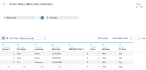
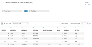
Our first example will use a few tiny tables about some people:
Four Types of Joins
Joins come in four different flavors: inner join, left join, right join, and full outer join. Each of these joins is created by using a common variable that is found in both tables. However, each of these joins creates a different connection (or sets up a different relationship) between the two tables. Let’s use the Children and Occupation tables to see how each of these joins works.
Inner Join
An inner join keeps only the records that appear in both tables.
In Tableau’s Data Source environment, connect to our Excel spreadsheet.
- Drag the Occupation Table into the orange area. You’ll see the Occupation Table appear below with just 4 variables: First Name, Age, Education, Occupation. There are five records: Wanda, Floyd, Clyde, Clyde, Betty. Clyde appears twice because he has 2 job titles.
- Remove the Occupation Table and add the Children table. You’ll see the Children table has 3 variables: First Name, Child and Age. Note that ‘First name’ links the 2 tables, but ‘Age’ does not. This was probably a back header name choice. It would have been better to make it ‘Child Age’ since the table is actually describing things about the adults – not the children. The children are the topic, but they are centered around the adults. We have 5 values Wanda, Wanda, Floyd, Clyde, Vincent. Note that Wanda appears twice, and we have someone new: Vincent. Betty seems to be missing. This is confusing because there are 2 possibilities: 1. She doesn’t have children (where it should be represented by 0 and NA) or 2. We don’t know her well enough yet, in which case, that should be more clearly indicated. The same is true for Vincent in the careers tab. Anyhow, this makes a good test set because people appear in one table but not the other.
- Now join the Children Table to the Occupation Table. Drag the Children Table into the same space where the Occupation Table already sits. Notice that Tableau immediately connects the two tables with an Inner Join represented by the venn diagram with just the center filled in. But nothing appears. This is because Tableau guessed which was the common column. It guessed wrong. Click on the circle to select the common column (First name)
- Now look that the data below. Both Vincent and Betty disappeared. An inner join only keeps records that appear in both tables. Since Vincent doesn’t exist in the Occupation Table, the record in the Children Table is dropped. Since Betty doesn’t exist in the Children table, her record in the Occupation table is dropped.
Inner joins are very common and can be a great way to limit your dataset to just records that appear in both places. For example, in our email example before, an inner join between your email table and contact table would drop all the emails for which you didn’t have a contact records, and would also drop all contact records who hadn’t sent you an email.
Left Join
A left join keeps all the records in the primary (left) table and drops unmatched records in the secondary (right) table.
Now click on the venn diagram icon in Tableau and change the join type from an inner join to a left join. Betty reappears. You’ll see that Tableau has added null in each cell for the Children Table variables since there is no information corresponding to her. However, Vincent still doesn’t appear because he doesn’t have a corresponding record in the Occupation Table.
A left join holds on to all of the records in the primary table on the left (all the Person records) and the looks to the right table for any corresponding information. Left joins are also common. Continuing with our email / contact example, a left join would hold onto all of the email records, match up any corresponding contacts, and just create null values for anyone who wasn’t in your contacts. Anyone who was in your contacts but didn’t send you an email would be dropped.
Right Join
A right join keeps all the records in the secondary (right) table and drops all unmatched records in the primary (left) table.

A right join functions just like a left join in reverse. Change the join in Tableau and you’ll see Betty disappear and Vincent appear. All the records in the secondary table on the right are kept and matched up to any corresponding records in the left table.
Right joins are much less commonly used, mainly because if you actually cared about the table on the right more than the table on the left, you’d drag that table out first and create a left join instead. In our email/contacts example, a right join would create a dataset with all of your contacts and would only keep the emails for which you had a contact record.
Full Outer Join
A full outer join keeps all the records in both tables.

Last but not least, change the join type to full outer. You’ll see the entire venn diagram icon filled in. All records from both tables will be kept and any missing values will just be filled in with null. This means that Betty from the Occupation Table appears even though isn’t in the Occupation table, and Vincent from the Children Table appears even though he doesn’t have an Occupation in the table. In our email example, this would mean all of your emails and all of your contacts would be included in the dataset.
Maintenance and Flexibility of Smaller Tables
You can, of course, add more tables so long as there is a unique identifier to join on. Imagine we had an income table and we had joined them all together. Now Think of updating this dataset once someone gets a new job, has a kid, or gets a raise. It’s much easier to just go to a smaller table with only that information and add a few new pieces of information than it would be to update all of the other unrelated information in this bigger table.
It also makes your data much more flexible. Let’s say you just wanted to look at the Occupation and the Salary tables. You wouldn’t have the mess with the Children data at all. Smaller tables like this make it much easier to only work with the data you need.
UN Data: Joining on Multiple Variables
Now let’s move on to a more realistic example of when you’ll use joins. Go to the UN’s Population Division’s Download Center and toggle over to CSV format. This is where the two UN tables in today’s Excel Workbook come from. Take a look at the instructions to combine tables: “Use the LocID, VarID and Time columns to link the data across the different files, if necessary. Note that Time differs between single year (e.g. 1950) and period (e.g. 1950-1955) data.” These are our join instructions.
In order to connect these two tables, we have to join on multiple variables. Take a moment and think about why. If we connect population data for multiple years.
Let’s use this information in Tableau.
Joining real data
Download the Demographic Indicators – Medium variant (the zip file as a csv in it). We want to be able to visualize the relationship between overall population of a country and factors such as birth and death rates. Note that the Population data is annually whereas the Period indicators are every Five years. If we do an inner join, what do you expect to happen?
If we do a left join, what do you expect to happen? Why
These are csv files and therefore only have 1 tab each. Load each file separately and then join them both ways. Did what you predicted happen?
Now go back to the inner join because that actually tells us the most information. In a real project, we would rename those column names to something more descriptive.
- When we do an inner join, the tables join on the LocID. This is great, but causes redundancy that we don’t want. We also need to incorporate the year somehow.
- The Indicators table is in 5 year increments, but the Population by Sex table is in 1 year increments. What do we do? We’re going to use the Year variable from the Population by Sex table, and the Midpoint variable from the Indicators table.
- Click on the Join and add a new row to join on. You should get an error message. This means that the datatypes of these two variables are not the same. If we inspect the Midpoint, we see it’s a decimal number whereas the Year is a whole number. We want to change to the more specific, so we’ll make the decimal the year.
- Congratulations!! You have successfully joined your datasets. Now we will visit our datasheet to make a visualization of Net Migration.
- Drag the Time Pill to the Columns and the Net migration Pill to the Rows and the Location Pill to the Rows. This is too many countries. We need to look at fewer.
- Filter for just the US, China, and the BRIC countries (Brazil, Russia, India, China) to better understand the migration patterns of these economically important countries.

